Learning Differentiable Decision Trees for Reinforcement Learning: Q-Learning or Policy Gradient?
In conjunction with an earlier post on the use of Differentiable Decision Trees (DDTs) for interpretable reinforcement learning, this post will cover my recent AISTATS paper Optimization Methods for Interpretable Differentiable Decision Trees in Reinforcement Learning. In my earlier post, I laid out some reasons that we might want to use DDTs for reinforcement learning: they afford discretization for interpretable plans, they allow for warm-starting and human initialization, and they are surprisingly robust to hyperparameter selection (things like learning rates, number of layers, and so on).
Our Problem
Assuming we want to deploy a DDT to reinforcement learning, we need to somehow learn the optimal parameters. Here we have a choice: policy gradient approaches, or Q-learning approaches? Both have shown promise across the field, and so we run a comparison on the effects of using them with DDTs. Our problem setup is simple:

Our 4-state MDP for evaluating Q-Learning and Policy Gradient in DDTs. The agent receives reward for being in the middle states, so the optimal policy is one that moves left from S3 and right from R2.
We consider a standard Markov Decision Process (MDP) with 4 states [1]. Each run, agent starts in either S2 or S3, and gathers positive reward while it stays in one of those two states. However, the episode ends if the agent reaches S1 or S4. From this, it follows pretty clearly that the agent should always move right from S2, and move left from S3. If we were to put together a decision tree for this problem, we could do it pretty simply with just one node.
The MDP Solution:
The optimal tree for this 4-state MDP is given in the image on the right. If you look at it for a minute, it should make sense. If the state is greater than 2.5 (meaning we’re somewhere on the right side of the chain), we should move left. If that isn’t true, and the state is less than 2.5 (we’re somewhere on the left side of the chain), then we should move right! This keeps the agent bouncing back and forth in the middle of the MDP, alive and accruing reward.
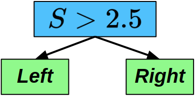
The optimal decision tree for our 4-state MDP, where “True” corresponds with moving left down the tree, and “False” corresponds with moving right down the tree.
Finding the Solution:
So we know what the solution should be for this MDP, what happens if we put together a simple 1-node DDT and drop it into this problem? We’ll assume that the tree is pretty well-structured already— True will evaluate to “Left”, False will evaluate to “Right”, and so we just want to know: which value should we be checking the state against? Put another way: what is the splitting criterion? The optimal setting is 2.5 [2], so what will Q-Learning and Policy Gradient decide it should be?
Q-Learning
To figure out where Q-Learning might take our DDT, we plot out the parameter update for all of the different possible splitting criteria between 0 and 5. What we want to see is that the gradients of these updates are only zero in one place— 2.5. These zero-gradient points are called critical points, and they’re places where the model would stop updating its parameters (meaning it would consider itself finished training). Everywhere else, there should be some gradient, however small, nudging the parameters towards these critical points.
So what does that turn out to look like for Q-Learning?
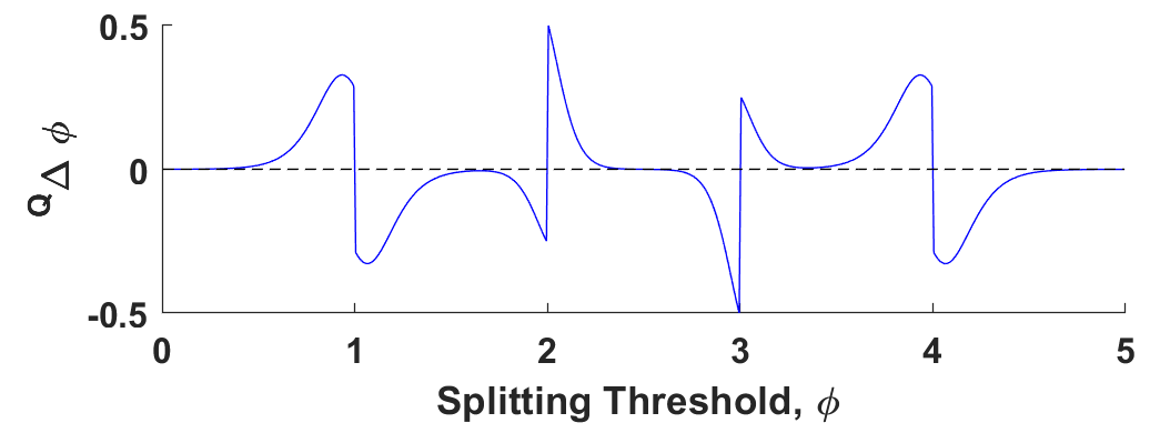
Critical points for Q-Learning applied to our 1-node DDT. As we can see, Q-Learning exhibits pretty substantial instability for learning this model’s parameters, presenting us with 5 zero-gradient options, only 1 of which is coincident with the optimal setting of 2.5.
Yikes.
It turns out that Q-Learning presents us with 5 critical points, only one of which is coincident with 2.5. The other 4 are all sub-optimal local minima— places that the model would stop updating but which clearly do not present us with an optimal solution.
Policy Gradient
With Q-Learning examined, what about Policy Gradient approaches? We set the problem up the same way: plot gradient updates for all values of S between 0 and 5 and look for critical points— points that have zero-gradient.

Critical points for Policy Gradient applied to our 1-node DDT. As we can see here, Policy Gradient is significantly more stable for this problem, presenting with only one critical point which is nearly exactly on 2.5.
Policy Gradient is so much more stable! For this problem, there is only one critical point, which is nearly exactly coincident with 2.5, the optimal setting.
The Takeaway
The takeaway from all of this is: if you’re going to work with DDTs in reinforcement learning, you should be training your agents with policy-gradient approaches rather than Q-Learning approaches. Policy gradient exhibits greater stability, more closely reflects the ground truth of the problem, and works well empirically! For the full details, have a look through the paper!
[1]This may be extended to any number, but for simplicity, we’re going to stick with 4.
[2]For any number of states n, the optimal setting is: (n/2)+(1/2)