A brief foreword: This entire post is a high-level summary of the motivations and contributions of my paper which was recently accepted to AISTATS 2020! For some math on why Q-Learning is less stable than policy gradients for differentiable decision trees, a full list of my references/sources, and more thorough comparisons, etc. check out the full paper: Optimization Methods for Interpretable Differentiable Decision Trees in Reinforcement Learning.

Why aren’t normal neural networks interpretable?

In my last post, I wrote about why we want interpretability and what that means. But why is it something that’s so hard, and why aren’t normal methods just easier to understand?

Ultimately, neural networks are lots of matrix multiplication and non-linear functions in series. And following where a single number goes and how it affects the outcome of a set of matrix multiplication problems can be rather daunting.

One of my agents on the cart pole problem in the OpenAI Gym

In some of my recent work, I trained a simple neural network agent to solve the cart pole problem from the OpenAI Gym. The objective of the challenge is to balance an inverted pendulum (the pole) on a cart that can shift left or right on a line. By just nudging gently left and right, it’s possible to keep the pole balanced upright.

While the system works out just fine, if you wanted to visualize the network’s decision-making process, it wouldn’t be so easy. Then again, cart pole is a simple problem:
There are only four variables in the state, and a network with two layers can solve the problem.

Perhaps the closest you could get is to draw out all of the different matrix multiplication operations that would need to take place, and then try to trace through the math each time. With such a simple problem and network, maybe that isn’t so bad?

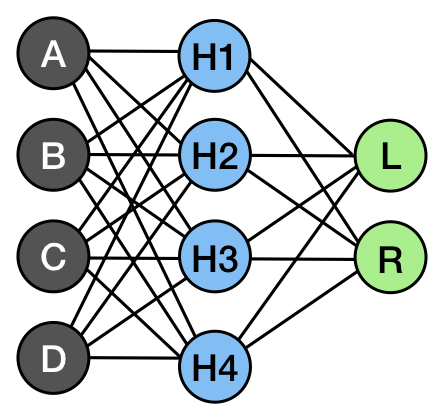
Here’s the usual drawing of a neural network. Our inputs are A, B, C, D, and they go to a single layer of hidden units H1, H2, H3, and H4, before being passed to the output units (Left or Right).

A drawing of the weights for a two-layer multi-layer perceptron on the cart pole problem. For reference, A is the cart position, B is the cart velocity, C is the pole angle, and D is the pole’s angular velocity.

As it turns out, it’s completely ridiculous. I mean, just look at it. To know what the network would do in any given state, you need to be able to run through 4 quick matrix multiplication problems, save the results, run through 2 more matrix multiplication problems, and then compare the two results you get. I tried doing this for myself and I ended up giving up after spending several minutes and still getting the wrong answer. And this doesn’t even have non-linearities!

What about something like attention?

Attention is a very powerful and useful innovation in deep networks, and it can offer insights into which variables are meaningful and relevant. While that might be a useful tool for seeing which features matter, we want to see exactly what our network will do, not just know what it’s looking at.

With that in mind, let’s pretend we have attention in this single hidden layer network by saying that we just make each matrix multiplication instead only considers a single element. Would that make matters simpler?

If we make the above problem more “one-hot” it still doesn’t end up in the friendliest of places…

So, yes, it has made things simpler. But the notion of following this set of matrix multiplications in some sort of critical scenario is still ridiculous. Walking through all of this math just to know what my robot is going to do is absolutely not something I want to be doing. And even if it is possible to quickly see what will happen in a given state, a model like the one above is not prescriptive. I can’t use that model to quickly tell you what to expect from my robot as it navigates around the world, I can only tell you what output you’ll get from a particular input. Not only that, but this discrete-neural-network approach would perform terribly on something like the cart pole problem up above.

So what about differentiable decision trees?

Decision trees are a more classic machine learning approach which yield interpretability, simplicity, and ease of understanding. The actual format of a decision tree is essentially a list of “Yes or No” questions until the machine finally arrives at an answer.

Going back to cart-pole up above, we might say “If you’re to the left of center, move right. Otherwise, move left.” If we know that:

“A” is the cart position,
0 is center, and
negative is left,

then this is a very simple decision tree which could be drawn like so:

If A is our position, 0 is the center, and left is negative, and the left arrow is “True” and the right arrow is “False”, then this perfectly captures: “If left of center: move right. Otherwise: move left.”

Now, this is a bit simplistic and in reality it wouldn’t actually do very well. There is a trade-off here between simplicity and performance. The crazy complicated matrix math does quite well, but we can’t understand it. The dead-simple decision tree is very easy to understand, but it doesn’t do all that well. Can we combine the two?

As it turns out, yes! By structuring a network like a decision tree, we can learn how to perform well in a reinforcement learning environment, and then have all of the network’s “knowledge” captured in a convenient decision-tree shape. That doesn’t quite solve our matrix math problem, but it gets us closer.

Instead of a multi-layer network with obscure mappings and math, we have simpler single-layer checks which spit out a “True” or “False,” and eventually a very small pair of weights on different actions. Each check is itself a layer of the network, and the outputs are themselves sets of parameters. So instead of a multi-layer network like this:

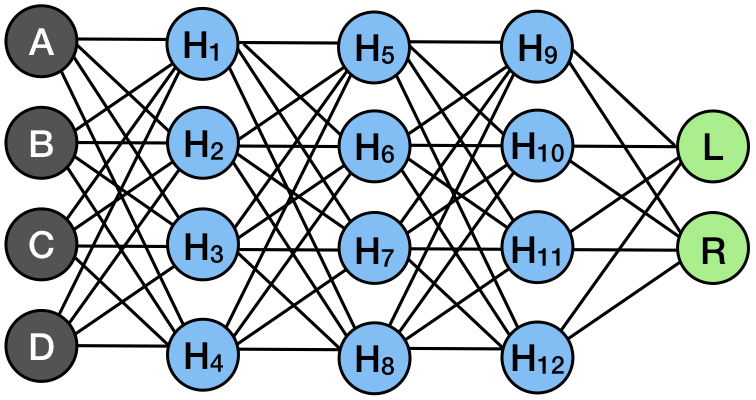
A multi-layer perceptron which would be rather nightmarish to manually follow through every input to trace out how we got the actions we got.

We can sort of decompose our network into mini sub-networks, where each mini-network is a single decision in the tree.

Each layer in the network can be seen as a mini-network which makes a single choice: True or False?

Okay, so this isn’t that much simpler yet. We got rid of a nasty set of repeating hidden layers which would have been a pain to follow, but we still don’t want to figure out how each of these works in order to understand the entire system. So next up, we return to that idea of attention and simplifying layers of the network.

While training, the network is allowed to make use of all of its hidden units and learn the best solution possible. However, when it finishes training, we take advantage of attention to choose just a single variable to care about. Not one hidden unit, just one input variable (like the cart position, A, for example). When the layer is only looking at one variable, we can actually just collapse all of the math into a single operation, multiplying by one weight and adding one bias. So taking one of the mini sub-networks above, we convert it like so:

We start with a whole single-layer network, then we simplify into a single-variable network, and then further into a single-operation network

Now, we simplify even further and just convert the single operation into a simple check against the variable we care about (in this case, A). Then, we’ve successfully converted a mini sub-network into a piece of a decision tree!

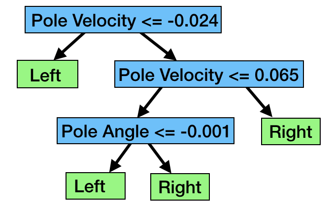
When we repeat the process, we can convert any of our differentiable decision trees into ordinary decision trees. They can learn complicated and obscure ways to solve problems, but we can always convert them back into interpretable and clean decision trees to see how they work. To show an example, here is one that was able to nearly perfectly solve the cart-pole problem:

Cleaning up the [A, B, C, D] notation, this is one of the decision trees extracted from our approach for the cart pole problem

Compared to the matrix-multiplication headache of following a very simple neural network, this is cleaner and far more useful! We may still not have a great immediate understanding of what a pole angle > -0.41 really means, but there’s no denying that this is much easier to interpret than the original neural network.

Why not just use a normal decision tree, but bigger?

There are other ways to get a decision tree for most machine learning problems! We don’t need to go through this complicated process of training a neural network and then extracting a decision tree, we can just directly learn one from the data. If we have somebody demonstrate how to balance a cart on a pole, we can use that data to learn a tree without needing a neural network. I used a trained neural network to provide 15 “perfect” demonstrations and then learned a decision tree directly from those demonstrations, and here is the tree that came out:

Suspiciously small decision tree for cart pole using sklearn over a set of demonstrations.

Okay wow, that is still super simple. In reality, the tree that was returned was much larger, but so many of the branches or paths ended up being redundant (as in, a check leads to leaves that are all “Left”, so there was no reason to make the check in the first place) that I was able to manually simplify it to this format. And as you might expect, unfortunately, it’s very bad at solving cart pole. The tree above averaged a score of somewhere near 60, where the decision tree extracted from a neural network averages 499, and the neural network model averages 500, the top score. So in short: we don’t use decision trees directly because they’re very bad.

So where does that leave us?

If you want pure performance: a neural network. It’s always going to be a stretch for any simple, linear algorithm or model to match the performance of a complex deep network. If you’re okay with sacrificing a tiny bit of performance for a much simpler and easier to interpret model, the differentiable decision tree offers you both strong performance and very clear insight into the agent’s inner-workings. You’re also able to intelligently initialize differentiable decision trees, but that’s a story for another day.

Of course, enormous thanks to Taylor Killian, Ivan Dario Jimenez Rodrigues, Sung-Hyun Son, and my advisor Professor Matthew Gombolay. For more details, check out the full paper, and for more cool robotics and machine learning work, keep up with the CORE Robotics website!

Andrew Silva, Matthew Gombolay, Taylor Killian, Ivan Jimenez, Sung-Hyun Son ; Proceedings of the Twenty Third International Conference on Artificial Intelligence and Statistics, PMLR 108:1855-1865, 2020.